Climate sensitivity: where the numbers come from

Four quantities, four experiments, four ways of asking the same question

Dean Rovang · substack.com/@deanrovang · ORCID: 0009-0006-1351-5320

Abstract

Climate sensitivity is invoked as a single contested number, usually 3 °C, sometimes higher or lower. This framing dissolves once you understand that sensitivity is not one quantity but four — TCR, ECS, ESS, and the empirical paleoclimate slope (AESS). Each is the response of the climate system to doubled CO₂, measured at a different point in time, with different feedbacks allowed to express. Different numbers are not disagreement. They are the same physical response viewed at different stages of its unfolding. This essay walks through where each number comes from — what experiment defines it, what evidence constrains it, and how to recognize when an argument confuses one quantity for another.

Where the numbers come from

Zeke Hausfather has an excellent Carbon Brief explainer on climate sensitivity. It defines TCR, ECS, ESS. It names the three approaches the IPCC uses to combine evidence. It points to the AR6 likely range of 2.5–4.0 °C. After reading it, I still came away wondering exactly how the numbers themselves are derived.

That gap is what this essay is about. The vocabulary is well-explained elsewhere. What is harder to find in one place is a walk-through of what each quantity is and where its value comes from: which parts are analytically derivable, which require running climate models, which require observational measurements, and which come from plotting the data and fitting a line through it. Once these are separated, a whole category of disagreement about climate sensitivity dissolves — not because the disagreement is fake but because the disputants are often measuring different things.

Two figures anchor the essay. Figure 1 shows the CO₂–temperature relationship across 66 million years of paleoclimate data, the modern instrumental record, and the AR6 SSP2-4.5 projection through 2100. Figure 2 shows the same sensitivity quantities laid out as snapshots of a single response curve in time.

I. What the physics actually fixes

Two quantities in climate sensitivity come closest to falling out of pencil-and-paper physics.

The radiative forcing from doubled CO₂ (~3.7 W/m²). This is calculated from line-by-line radiative transfer through a known atmospheric profile. Not pencil-and-paper exactly — the calculation needs computational integration across thousands of spectral lines — but anchored to spectroscopy measured in the laboratory for more than a century. The Tyndall-Foote tradition, continued. The current best estimate has roughly 10% uncertainty depending on the assumed atmospheric water vapor profile and other inputs.

The Planck response (~1.2 °C). What the surface would warm by if the atmosphere had no feedbacks at all — only the adjustment of outgoing thermal radiation as the surface heats up. Derivable in closed form from Stefan-Boltzmann (a warm body radiates more), with one caveat: the exact value depends on what you hold constant. The conventional value is 1.2 °C per doubled CO₂.

These two quantities together account for roughly 10% of the predicted long-term warming. They are the most analytically transparent values in climate science. Everything else — the path from 1.2 °C to roughly 3 °C, and from 3 °C to roughly 8 °C — comes from feedbacks expressing on different timescales. Each feedback amplifies or dampens the initial response. Their combined effect, and the time over which they express, is what produces the four sensitivity metrics.

II. Four metrics, four experiments

The four sensitivity quantities are defined by what experiment is performed and when the temperature is read.

TCR (Transient Climate Response, ~1.4–2.2 °C). The experiment: increase CO₂ at 1% per year until it doubles (year 70), then read the average temperature for years 61–80. TCR captures water vapor feedback, lapse rate feedback, the part of cloud feedback that has expressed in 70 years, and the modest sea-ice retreat that fits in that interval. The deep ocean has barely begun to warm. Slow feedbacks (ice sheets, vegetation) have not started.

ECS (Equilibrium Climate Sensitivity, AR6 likely range 2.5–4.0 °C, central estimate ~3.0 °C). The experiment: hold CO₂ at 2× preindustrial and wait until the system stops adjusting. In practice, models quadruple CO₂, run for 150–300 years, and extrapolate to equilibrium. ECS includes everything in TCR plus full cloud feedback, full sea-ice response, and the deep ocean’s slow warming. It still excludes ice sheets, vegetation, and the slow carbon cycle by definition.

ESS (Earth System Sensitivity, ~5–8 °C). The experiment: hold CO₂ at 2× preindustrial and wait longer — millennia. Now ice sheets retreat, boreal forests march north, soil and vegetation reorganize, and ocean carbonate chemistry adjusts. All of this further amplifies warming. ESS is harder to estimate than ECS because the experiment is harder to model. Coupled ice-sheet and dynamic-vegetation models are newer and less well-validated than the atmosphere-ocean models used for ECS.

AESS (Apparent Earth System Sensitivity, ~8–9 °C). The experiment: don’t run a model at all. Plot atmospheric CO₂ against global temperature for the available paleoclimate data and measure the slope. This is the equilibrium relationship visible in Figure 1, traced out over millions of years across multiple independent archives. The word apparent is doing work: the slope is what is observed, not a clean separation of CO₂’s response from everything else that was changing over geological time. For the question of where the system is likely to land if a CO₂ level is sustained for many millennia, AESS is the most directly observational quantity available.

The gap between ESS (~5–8 °C) and AESS (~8–9 °C) is real and worth naming. ESS as computed by Earth System Models captures the slow feedbacks that current models include: ice sheets, vegetation reorganization, ocean carbonate chemistry on millennial timescales. AESS captures everything that actually happened in the paleoclimate record, which includes processes operating over hundreds of thousands of years — silicate weathering (the geological CO₂ thermostat, atmospheric CO₂ reacting with rocks to form carbonate minerals), full reorganization of vegetation and soil carbon pools, polar amplification effects that strengthen in sustained warm states, and state-dependent feedbacks where sensitivity itself rises in warmer climates (Anagnostou et al. 2016, Cael et al. 2026). The gap is the part of the long-term response that the modeled ESS does not yet fully capture. The reason to use AESS for paleoclimate questions is that the record measured all of it directly, regardless of whether models can yet reproduce the underlying mechanisms.

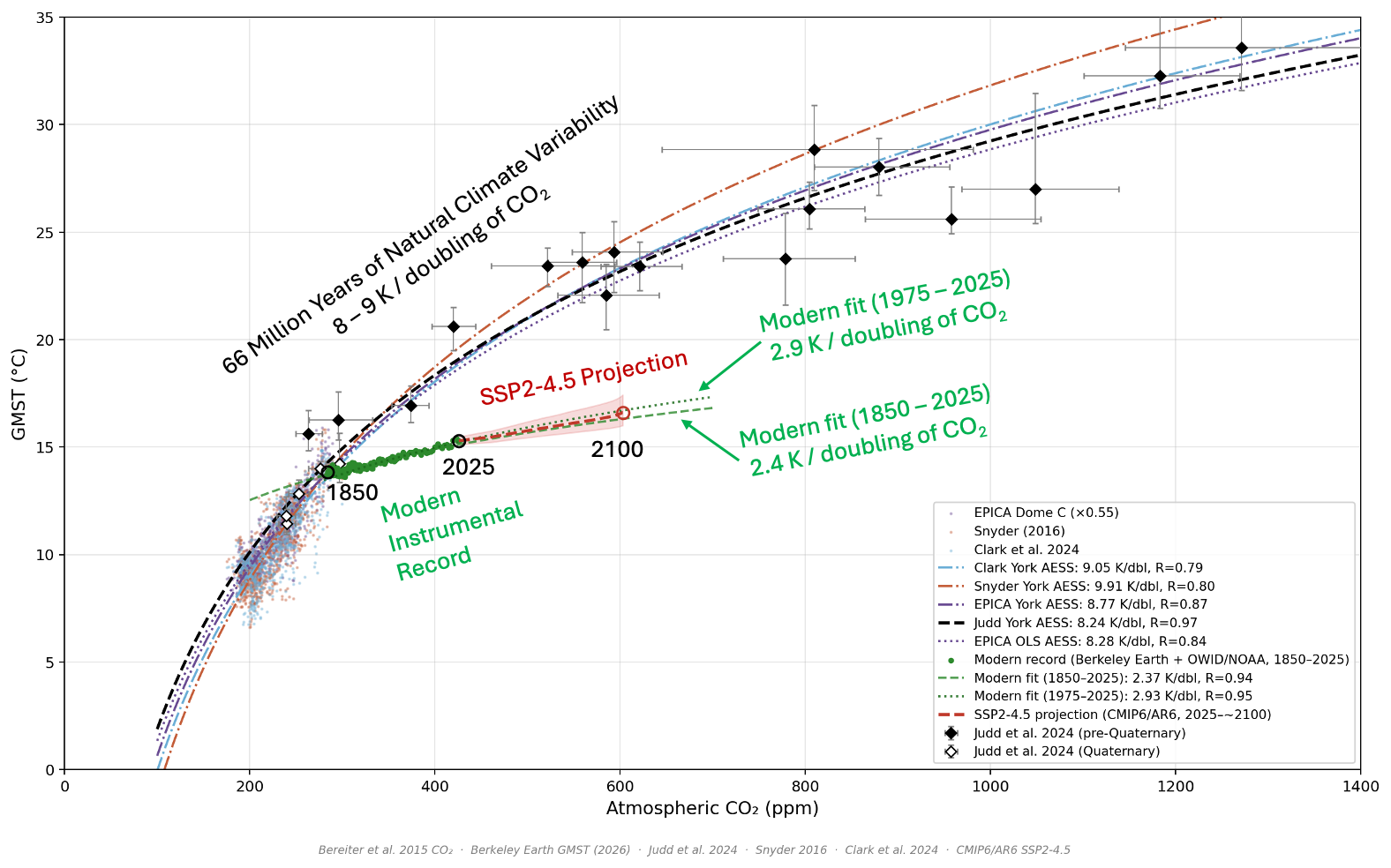
Figure 1. Global mean surface temperature versus atmospheric CO₂ across 66 million years of paleoclimate data, the modern instrumental record, and the SSP2-4.5 projection through 2100. The five paleoclimate regression fits (Clark, Snyder, EPICA York, Judd, EPICA OLS) cluster in the 8.2–9.9 K per doubling range — the AESS tier. Snyder (2016) is the high-side fit at 9.9; the AESS band quoted in the text and in Figure 2 (8.2–9.1) excludes it as an outlier and is taken from the other four regressions. The modern instrumental record sits in a distinct lower tier: the 1850–2025 OLS fit gives 2.37 K per doubling; the 1975–2025 fit gives 2.93 K per doubling. The two tiers are separated by an unfilled gap that the four-tier framework predicts — the transient response sits well below the equilibrium response, and the gap closes as forcing accumulates and slow feedbacks express. Data sources: Bereiter et al. 2015, Berkeley Earth, Judd et al. 2024, Snyder 2016, Clark et al. 2024, Meinshausen et al. 2020 (CMIP6/AR6 SSP2-4.5).

III. Four snapshots of one response curve

The four metrics are not four different theories of climate. They are four moments in the same response. Figure 2 shows this directly: a single curve of temperature versus time after CO₂ doubling, with TCR at year ~70, ECS at centuries, ESS at millennia, and AESS as the empirical band from paleoclimate.

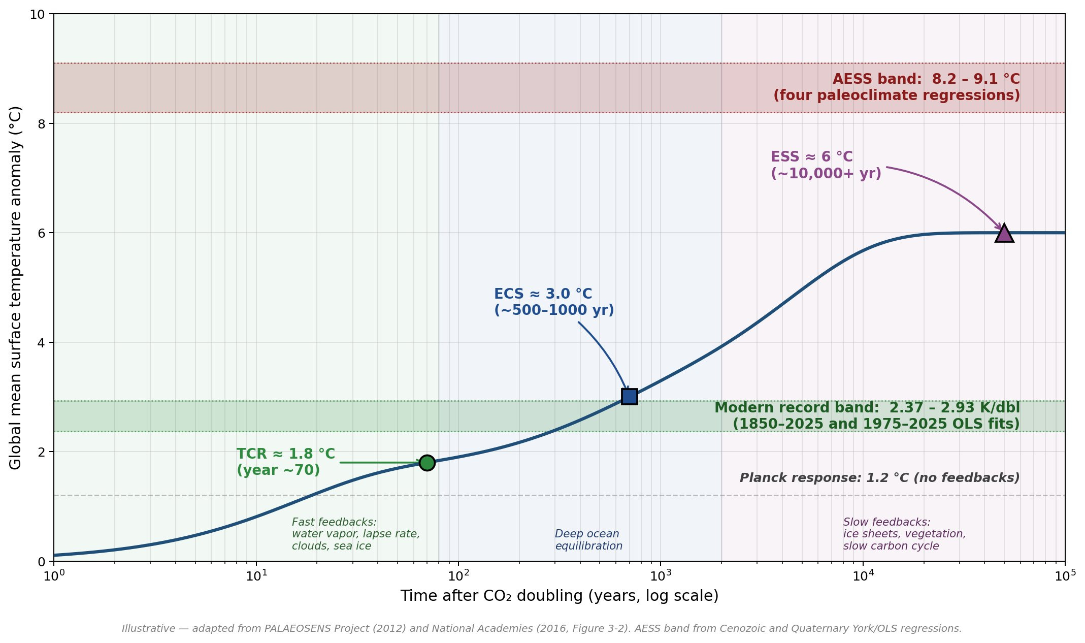
Figure 2. The climate system’s response to abrupt CO₂ doubling, plotted as temperature anomaly versus time (log scale). The blue curve is an illustrative three-component response model tuned to pass through TCR ≈ 1.8 °C at year 70, ECS ≈ 3.0 °C at centuries, and ESS ≈ 6 °C at millennia. Two empirical bands flank the curve: the AESS band at the top (8.2–9.1 °C, from four paleoclimate regressions) and the modern record band at the bottom (2.37–2.93 K per doubling, from the OLS fits to the 1850–2025 and 1975–2025 instrumental records shown in Figure 1). The Planck no-feedback response at 1.2 °C is shown as a dashed reference. Background shading marks the timescales over which different categories of feedback operate. ECS is shown at the AR6 assessed central estimate of 3.0 °C; the Appendix walks through how a single-stream feedback calculation gives 3.4 °C, and why the four-stream assessed value is lower. Adapted from PALAEOSENS Project 2012 and National Academies 2016.

The shape of the curve — fast initial response, plateau, then a second rise as slow feedbacks express — is what every climate model produces. The disagreements in the field are about the height of the plateau (the value of ECS) and the timing and magnitude of the second rise (the values and onset times of slow feedbacks). The disagreements are not about whether the structure exists.

The bands in Figure 2 are data. The top band is what 66 million years of paleoclimate record actually shows. The bottom band is what 175 years of the modern instrumental record actually shows. They are not theoretical claims about what the system ought to do. They are measurements of what it has done. The illustrative curve threading between them is one possible reconciliation — the response of the climate system as physics predicts. Whether the curve is exactly right in any detail is a separate question. The empirical bands are what they are.

Looking at the modern band specifically: it climbs. The 1850–2025 fit gives 2.37 K per doubling. The 1975–2025 fit gives 2.93 K per doubling. Foster (2026, Geophysical Research Letters) used changepoint analysis after removing the influence of ENSO, solar variability, and volcanic forcing, and found the acceleration statistically significant. Forster and colleagues (2025) report attributed human-induced warming has risen to 0.27 °C per decade for 2015–2024 — well above the 0.18–0.20 °C per decade rate of earlier decades. The observation is consistent with what the four-tier framework predicts: as forcing accumulates and slow feedbacks begin to express, the transient slope climbs toward ECS. The recent slope sits just below the labeled ECS value on Figure 2.

IV. Four streams of evidence

Where do the IPCC’s likely ranges come from? AR6 combines evidence from four independent streams, weighted by formal Bayesian inference. Each stream alone gives a wider uncertainty than the combined estimate. The tightening of the AR6 likely range — from AR5’s 1.5–4.5 °C to AR6’s 2.5–4.0 °C — came from this combination.

Stream 1: Physics plus models. Start with the 3.7 W/m² forcing and the 1.2 °C Planck response. Add feedbacks as parameterized in Earth System Models. Run the abrupt-2× experiment, extract ECS via linear extrapolation of the early temperature trajectory to the radiative equilibrium point (the Gregory method). Different models produce different ECS values — 1.8 °C to 5.6 °C across the CMIP ensemble — because they parameterize cloud and aerosol microphysics differently. The spread is honest; it is not error.

Stream 2: Observational energy budget. The CERES satellites have measured the planetary energy imbalance at the top of the atmosphere since 2000 (currently ~+0.9 W/m² in recent years). Combined with the surface temperature record and best estimates of historical forcing, this gives a feedback parameter and therefore an estimate of ECS that does not require running a climate model. Earlier work using this method produced lower ECS estimates (~2.0–2.4 °C). The gap turned out to be a methodological issue: the warming so far has been concentrated in regions whose cloud response does not represent the long-term equilibrium response — the so-called pattern effect. Cooper et al. (2026) corrected for pattern effects and brought observational ECS estimates to about 2.8 °C, consistent with the model-based estimates. The convergence between methods, once properly calibrated, is one of the more important developments in the last decade of climate science.

Stream 3: Paleoclimate. The deep past gives independent estimates. Warm states such as the Pliocene and Eocene constrain sensitivity at elevated CO₂. Glacial-interglacial cycles constrain it at lower CO₂. These estimates are noisier than the modern energy budget because both temperature proxies and CO₂ reconstructions carry error bars, but the central tendency is consistent with ~3 °C ECS for modern conditions, with higher values at warmer climate states. The formal framework for combining fast and slow feedbacks across paleoclimate was developed by the PALAEOSENS Project (2012, Nature).

Stream 4: Emergent constraints. Across models, certain present-day observables (cloud properties, the seasonal cycle, the response to volcanic eruptions) correlate with the model’s ECS. Apply the observed value to the model-derived relationship and you get an observationally-anchored constraint on ECS. Sherwood et al. (2020) combined multiple emergent constraints with the other streams in a formal Bayesian framework — the work that became the basis for AR6. More recent emergent-constraint work has continued to refine the picture. Wilson Kemsley et al. (2026, GRL) used satellite cloud observations to constrain cloud feedback and found it robustly positive, pushing the central ECS estimate modestly upward from AR6’s 3.0 °C.

AR6’s 2.5–4.0 °C likely range is what falls out when these four streams are combined. Each stream alone gives a wider uncertainty; the combination is tighter than any single stream. This is consilience working: multiple independent methods, with independent assumptions and independent failure modes, converging on overlapping ranges.

V. A worked example: the Hansen ECS

The framework’s real use is taking apart a dispute that usually arrives as a single tangled claim. James Hansen and collaborators argue for an ECS of roughly 4.5 °C or higher, well above the AR6 central estimate. It is tempting to file this as Hansen using a looser definition — letting ice sheets sneak into ECS — but that is not what is happening, and the framework is precise enough to show why.

Hansen’s 4.8 °C is, by his own paper’s label, a Charney (fast-feedback) sensitivity: the same experiment AR6 runs, with ice sheets and the other slow feedbacks held fixed. It is not Earth System Sensitivity, and it is not a hybrid sitting partway up the curve. It is an estimate of the same quantity AR6 puts near 3 °C — and it simply disagrees about the value.

Two choices produce the higher number, both inside the fast-feedback experiment. First, Hansen reads the fast feedbacks — cloud feedback above all — at the strong end of their range. Appendix D shows the consequence directly: with cloud feedback at +0.7 W/m²/K and ice sheets held fixed, the arithmetic gives ECS ≈ 4.6 °C. No slow feedback is needed to reach Hansen’s neighborhood; strong clouds alone get there. Second, he assesses historical aerosol forcing as more strongly negative than AR6 does. Aerosols mask greenhouse warming, so a larger hidden cooling means the observed warming was produced by a smaller net forcing — which implies a more sensitive system.

There is a second Hansen argument, and it is the one most often confused with the first. He reads the paleoclimate record as showing that the slow feedbacks — ice-sheet retreat in particular — and the warming already “in the pipeline” arrive faster than AR6 assumes, on the order of a century or two rather than millennia. This is a real and consequential claim. But it is a claim about how quickly ESS is realized, not about the value of ECS. One concerns the height of the fast-feedback plateau; the other, the timing of the slow rise. They are different axes, and Hansen’s critics and defenders routinely argue past each other by collapsing them into one.

The framework does not resolve whether Hansen is right on either count. On the fast-feedback value, the recent weight of evidence — the pattern-effect correction of Cooper et al. (2026), the four-stream AR6 assessment — sits near 3 °C, with Hansen on the high tail rather than at the center. On the speed of the slow response, the question is genuinely open. What the framework gives the reader is the ability to say whichdisagreement is on the table. That alone is more than most climate writing offers.

VI. What to ask when someone gives you a number

When someone tells you climate sensitivity is X, the productive question is not whether X is high or low. It is which experiment defines X.

Five sub-questions follow.

Which metric? TCR, ECS, ESS, AESS, or something between?

Which stream of evidence? Physics plus models, observational energy budget, paleoclimate, emergent constraints, or some combination?

Which feedbacks are included? Fast only, fast plus slow, all of them?

Over what timescale is the response read? Decades, centuries, millennia, geological?

How does the result compare to the other streams? An estimate from one method that disagrees with all the others is interesting but not yet authoritative; it has to survive consilience with the rest.

A reader who can apply this checklist is no longer susceptible to the framing that climate sensitivity is one contested opinion. It is a calculated quantity tied to specific experiments. The experiments are well-defined. The methods are published. The results are reproducible. The convergence across streams is the most important fact in the field.

VII. Data and fits of things that have been

Figure 1 and Figure 2 share a useful feature: they are largely empirical. The paleoclimate band, the modern record band, the response curve threading between them — these are data and fits of things that have been.The bands are what they are. The slopes are what the data give. If they tell us that the climate system has a four-tier response structure spanning short-term transient response to long-term equilibrium, that is what the record shows, regardless of which model framework or scenario we prefer.

The framework’s value is not that it gives a single right answer. It is that it makes the questions you can ask sharper. When AR6 says ECS likely falls between 2.5 and 4 °C, the reader now knows what experiment that range refers to. When Hansen says ECS is closer to 4.5 °C, the reader can recognize it as a high-end estimate of the same fast-feedback quantity AR6 centers near 3 °C — driven by strong cloud feedback, not by slow ones — and keep it separate from his distinct claim that the slow response arrives faster. When recent observational work shifts the central estimate modestly upward, the reader can place it in Stream 4. When the modern slope climbs from 2.37 to 2.93 K per doubling over the past 50 years, the reader can read that as the response curve doing exactly what physics predicts.

The climate science community has spent decades developing the methods that produce these numbers. The numbers are not opinions. They are quantitative results from defined experiments, constrained by independent observations. The framework does not eliminate disagreement — it relocates it from “is the science settled?” to “which experiment are we discussing?” Once that question can be asked clearly, most of the public confusion dissolves.

Appendix: the feedback arithmetic

The body of the essay treated feedbacks qualitatively. This appendix shows the bookkeeping — the governing equation, the measured parameters, the satellite constraint, and one worked example. Nothing here requires more than algebra.

A. The decomposition equation

The framework is the one electrical engineers use for amplifiers with feedback. At equilibrium, a radiative forcing F (in W/m²) is balanced by the climate system’s radiative response. Each physical process contributes a feedback parameter λ_i, in watts per square meter per kelvin of surface warming. The Planck response, λ_P = −3.2 W/m²/K, is the baseline restoring term — the extra thermal radiation a warmer surface emits. Equilibrium warming is

ΔT_eq = F / ( |λ_P| − Σ λ_i )

with amplifying feedbacks entering as positive terms in the sum. Equivalently, in gain form,

ΔT_eq = ΔT_Planck / (1 − g), g = Σ λ_i / |λ_P|

which any reader of Bode will recognize as a closed-loop gain. The system is stable so long as g < 1, and the paleoclimate record shows that it is. One structural consequence matters for everything downstream: 1/(1 − g) is nonlinear in g, so symmetric uncertainty in the feedbacks maps into asymmetric uncertainty in ΔT_eq. This is why sensitivity estimates have always carried a fatter upper tail than lower tail (Roe & Baker 2007). The shape of the uncertainty is built into the algebra, not into anyone’s pessimism.

B. The feedback parameters

AR6 Chapter 7 central values, in W/m²/K:

Planck: −3.2. Stefan-Boltzmann applied to the observed temperature structure of the atmosphere. The best-constrained number in the set.

Water vapor: +1.8. Warmer air holds more water vapor (Clausius-Clapeyron, roughly 7% per degree), and water vapor is itself a greenhouse gas. Constrained by satellite humidity records and consistent behavior across models.

Lapse rate: −0.5. The tropical upper troposphere warms faster than the surface and radiates to space more efficiently, partially offsetting the water vapor amplification. The two are often quoted as a combined +1.3 because their uncertainties anticorrelate — the same upper-tropospheric moistening that strengthens one strengthens the offsetting other.

Surface albedo: +0.4. Retreating snow and sea ice darken the surface. Constrained by the observed retreat over the satellite era.

Cloud: +0.4 ± 0.3. The dominant uncertainty in the whole problem. Constrained by cloud-controlling-factor analyses against satellite observations; Wilson Kemsley et al. (2026) find it robustly positive.

C. What CERES actually measures

The CERES instruments have measured the net radiative imbalance N at the top of the atmosphere since 2000 — currently about +0.9 W/m². Out of equilibrium, the energy budget reads

N = F − λ ΔT

energy absorbed minus energy restored. Rearranged, λ = (F − N)/ΔT. Every term on the right is measured or independently estimated, so the feedback parameter — and from it ECS = F_2×/λ — comes out of observations with no climate model in the loop. Round historical numbers (net forcing to date F ≈ 2.7 W/m², N ≈ 0.9, ΔT ≈ 1.3 °C) give λ ≈ 1.4 W/m²/K and ECS ≈ 2.6 °C — the neighborhood of the energy-budget estimates that ran below the model range for a decade. (Forster et al. 2025 estimate F closer to 2.9 W/m² for 2024, which shifts the illustrative ECS down to about 2.4 °C; the qualitative point is the same.) The largest single uncertainty in this calculation is the historical aerosol forcing — anthropogenic aerosols partially offset CO₂ warming, so F is a net of greenhouse warming minus aerosol cooling, and the aerosol term is the least well-constrained piece. Beyond that, the pattern effect from Stream 2: the λ inferred from the historical warming pattern overstates the long-run restoring strength, because the warming so far has been concentrated in regions whose cloud response is unusually stabilizing. Correcting for it (Cooper et al. 2026) brings the observational estimate to about 2.8 °C.

D. A worked example

Sum the central feedbacks: Σ λ_i = 1.8 − 0.5 + 0.4 + 0.4 = +2.1 W/m²/K. The denominator is 3.2 − 2.1 = 1.1, and with F = 3.7 W/m² for doubled CO₂,

ΔT_eq = 3.7 / 1.1 ≈ 3.4 °C.

In gain form, g = 2.1/3.2 ≈ 0.66 and 1.2 °C / (1 − 0.66) gives the same answer. Two things are worth noticing. First, the single-stream feedback arithmetic lands near 3.4 °C — slightly above the AR6 assessed central of 3.0 °C shown in Figure 2. Both are correct; they answer different questions. The 3.4 °C is what one method produces from central feedback values. The 3.0 °C is the four-stream Bayesian assessed central, which pulls the estimate down and tightens the range. The difference between them is exactly what consilience does. Second, run the cloud feedback across its published ±0.3 uncertainty: at +0.1 the denominator is 1.4 and ECS ≈ 2.6 °C; at +0.7 it is 0.8 and ECS ≈ 4.6 °C. One parameter, at its published uncertainty, spans the entire AR6 likely range. That is the cloud problem in one line of arithmetic — and the reason Streams 2 through 4 exist: they constrain ECS in ways that do not require knowing the cloud feedback first.

Selected references

Anagnostou, E. et al. (2016). Changing atmospheric CO₂ concentration was the primary driver of early Cenozoic climate. Nature 533, 380–384.

Cael, B. B. et al. (2026). State-dependence of climate sensitivity over 800,000 years. [working citation.]

Charney, J. G. et al. (1979). Carbon Dioxide and Climate: A Scientific Assessment. National Research Council, Washington, DC.

Cooper, V. T., Armour, K. C., Hakim, G. J., Tierney, J. E., Burls, N. J., Proistosescu, C., Andrews, T., Dong, W., Dvorak, M. T., Feng, R., Osman, M. B., & Dong, Y. (2026). Paleoclimate pattern effects help constrain climate sensitivity and 21st-century warming. Proceedings of the National Academy of Sciences. https://doi.org/10.1073/pnas.2511370123

Forster, P. et al. (2025). Indicators of Global Climate Change 2024. Earth System Science Data 17, 2641–2690.

Foster, G. (2026). Global warming has accelerated significantly. Geophysical Research Letters 53, e2025GL118804.

Hansen, J. et al. (2023). Global warming in the pipeline. Oxford Open Climate Change 3, kgad008.

IPCC AR6 WG1 (2021). Chapter 7: The Earth’s energy budget, climate feedbacks, and climate sensitivity.

Judd, E. J. et al. (2024). A 485-million-year history of Earth’s surface temperature. Science 385, eadk3705.

Leach, N. J. et al. (2021). FaIRv2.0.0: a generalized impulse response model for climate uncertainty and future scenario exploration. Geoscientific Model Development 14, 3007–3036.

Loeb, N. G. et al. (2021). Satellite and ocean data reveal marked increase in Earth’s heating rate. Geophysical Research Letters 48, e2021GL093047.

Meinshausen, M. et al. (2020). The shared socio-economic pathway (SSP) greenhouse gas concentrations and their extensions to 2500. Geoscientific Model Development 13, 3571–3605.

Myhre, G. et al. (1998). New estimates of radiative forcing due to well mixed greenhouse gases. Geophysical Research Letters 25, 2715–2718.

National Academies of Sciences, Engineering, and Medicine (2016). Assessment of Approaches to Updating the Social Cost of Carbon: Phase 1 Report. The National Academies Press.

PALAEOSENS Project (2012). Making sense of palaeoclimate sensitivity. Nature 491, 683–691.

Roe, G. H. & Baker, M. B. (2007). Why is climate sensitivity so unpredictable? Science 318, 629–632.

Sherwood, S. C. et al. (2020). An assessment of Earth’s climate sensitivity using multiple lines of evidence. Reviews of Geophysics 58, e2019RG000678.

Wilson Kemsley, S. et al. (2026). Recent cloud controlling factor analyses indicate higher climate sensitivity. Geophysical Research Letters 53, e2025GL118366.